
Experimental design
There are three 3 tier-1 experiments, with the name of the experiment in bold. All three experiments for coupled climate models will start with a “reasonably equilibrated” preindustrial control simulation as the initial conditions. For OGCMs, initialization should take place after no less than five cycles of the CMIP6/OMIP atmospheric forcing.
1) SOMIP wind: An experiment that increases the winds over the Southern Ocean and shifts them poleward Implications via a surface ocean momentum flux perturbation: 1 run (100-300 years total).
2) SOMIP freshwater: An experiment where the stability of the Southern Ocean is changed via a 0.1 Sv external source of fresh water (so-called water hosing). Implications: 1 run (100-300 years).
3) SOMIP wind + freshwater: experiment will use both the increased wind forcing and the water hosing described above. Implications: 1 run (100-300 years).
The forcing will be applied for 100 model years in these perturbation experiments. If resources are available, the model should be integrated for another 100-200 years with the perturbation forcing continued.
All the experiments will add fixed (in both time and space) anomalies to the surface fluxes computed by the coupled climate model or earth system model (like a flux adjustment). The perturbation fluxes will only be applied to the ocean surface, not to the sea ice if present. The atmosphere has no direct knowledge of these altered winds or freshwater inputs. These surface flux perturbations (wind and/or fresh water) will be applied to the ocean and are constant in time for the first 100 years of each experiment.
The wind perturbations will have a defined latitudinal profile and the magnitude of the maximum perturbation will be approximately 50% of the unperturbed wind stress, similar to previous studies (Farneti & Delworth 2010; Farneti and Gent 2011; and Gent & Danabasoglu 2011).
The fresh water fluxes will have the same magnitude (0.1 Sv for 100 years) spread evenly around the coast of Antarctica, but we leave the actual method of applying the perturbation to each participating group: each can decide whether to spread it out in a band and/or put some or all of it into icebergs. A 0.1 Sv freshwater forcing is equivalent to roughly a 1 m/century increase on global mean sea level. DeConto and Pollard (2016) project this to be a late 21st century forcing under RCP4.5, or mid-21st century forcing under RCP8.5
The experiments will branch from and be analyzed by comparison with the standard CMIP DECK preindustrial control simulation. All the experiments should have fixed preindustrial atmospheric conditions.
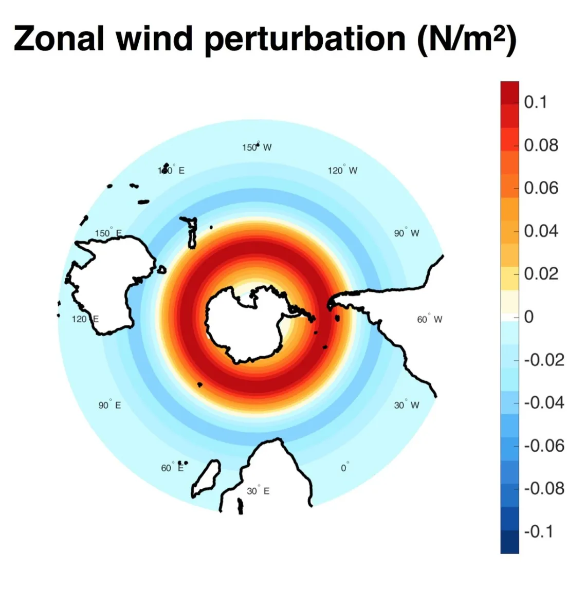
Zonal wind stress perturbation, where the maximum perturbation is designed to be ~50% of the unperturbed wind stress. The perturbation shown is the 60°S-15°S zonal and annual-mean of that imposed as part of FAFMIP. Note that experiments will differ slightly as we are imposing the perturbation, which will be added to the internally-calculated wind stress in a coupled model or to the wind stress forcing in an ocean/ice model.
The wind perturbations are the 90°-15°S zonal and annual mean of the zonal component of the FAFMIP wind perturbation. We have opted for a zonal mean profile because we are only using the FAFMIP perturbation south of 15°S in an idealized scenario. Our goal is force the westerly jet southward and increase its strength, not directly assess the response to projected wind stress perturbations like FAFMIP. Since the FAFMIP wind stress field varies zonally but the SOMIP one does not, we tested the bias introduced by taking a zonal mean. We compared the response of sea surface temperature, ocean heat content and sea level to the full FAFMIP wind stress forcing and the global zonal mean of the FAFMIP perturbation (run for 95 years as a step experiment):

One possible realization of the area over which the fresh water forcing perturbation will be added. We are proposing that a perturbation of 0.1 Sv be added, but will leave the specifics of the delivery method (fixed flux over a targeted area or delivery through icebergs released at discrete locations or some combination of the two) to each participant.
In the freshwater perturbation experiments, we will impose a standard size perturbation equivalent to an anomalous freshwater input of 0.1 Sv. Several previous studies have applied uniform anomalies around Antarctica, either out to 60°S (Seidov et al., 2005, doi:10.1016/j.gloplacha.2005.05.001) or closer to the coast (Aiken and England, 2008, doi:10.1175/2007JCLI1901.1). Several groups (notably van den Berk and Drijfhout, 2014, doi:10.1016/j.ocemod.2014.07.003) have suggested more realistic ice-melt scenarios where locations and amounts are based on the existing patterns of melt and flow, and there have been studies as to the effects of icebergs as a freshwater delivery mechanism (Martin and Adcroft, 2010, doi:10.1016/j.ocemod.2010.05.001).
If participating modeling centers have the time, inclination and resources, running an ensemble of perturbation experiments with differing initial conditions (with 5-member ensembles) will provide quantification of the size of the forced response to the perturbation and its significance relative to the pre-existing variability in each model.